kaggle dataset: Book Depository Dataset
kaggle notebook: Introduction to Book Depository Dataset
github repo: book-depository-dataset
Book Depository Dataset EDA
This notebook explores the Book Depository Dataset and extracts useful insights. The goal is to provide an introductory overview of the dataset.
import pandas as pd
import os
import json
from glob import glob
import matplotlib.pyplot as plt
import seaborn as sns
% matplotlib
inline
Dataset Structure
Files:
categories.csvdataset.csvformats.csvplaces.csv
The dataset consists of 5 file, the main dataset.csv file and some extra files. Extra files works as lookup tables for
category, author, format and publication place. The reason behind this decision was to prevent data redundancy.
Fields:
authors: Book’s author(s) (list of str)bestsellers-rank: Bestsellers ranking (int)categories: Book’s categories. Checkauthors.csvfor mapping (list of int)description: Book description (str)dimension_x: Book’s dimension X (floatcm)dimension_y: Book’s dimension Y (floatcm)dimension_z: Book’s dimension Z (floatmm)edition: Edition (str)edition-statement: Edition statement (str)for-ages: Range of ages (str)format: Book’s format. Checkformats.csvfor mapping (int)id: Book’s unique id (int)illustrations-note:imprint:index-date: Book’s crawling date (date)isbn10: Book’s ISBN-10 (str)isbn13: Book’s ISBN-13 (str)lang: List of book’ language(s)publication-date: Publication date (date)publication-place: Publication place (id)publisher: Publisher (str)rating-avg: Rating average [0-5] (float)rating-count: Number of ratingstitle: Book’s title (str)url: Book relative url (https://bookdepository.com +url)weight: Book’s weight (floatgr)
So, lets assign each file to a different dataframe
if os.path.exists('../input/book-depository-dataset'):
    path_prefix = '../input/book-depository-dataset/{}.csv'
else:
    path_prefix = '../export/kaggle/{}.csv'

df, df_f, df_a, df_c, df_p = [
    pd.read_csv(path_prefix.format(_)) for _ in ('dataset', 'formats', 'authors', 'categories', 'places')
]
# df = df.sample(n=500)
df.head()
| authors | bestsellers-rank | categories | description | dimension-x | dimension-y | dimension-z | edition | edition-statement | for-ages | ... | isbn10 | isbn13 | lang | publication-date | publication-place | rating-avg | rating-count | title | url | weight | |
|---|---|---|---|---|---|---|---|---|---|---|---|---|---|---|---|---|---|---|---|---|---|
| 0 | [1] | 57858 | [220, 233, 237, 2644, 2679, 2689] | They were American and British air force offic... | 142.0 | 211.0 | 20.0 | NaN | Reissue | NaN | ... | 393325792 | 9.780393e+12 | en | 2004-08-17 | 1.0 | 4.24 | 6688.0 | The Great Escape | /Great-Escape-Paul-Brickhill/9780393325799 | 243.00 |
| 1 | [2, 3] | 114465 | [235, 3386] | John Moran and Carl Williams were the two bigg... | 127.0 | 203.2 | 25.4 | NaN | NaN | NaN | ... | 184454737X | 9.781845e+12 | en | 2009-03-13 | 2.0 | 3.59 | 291.0 | Underbelly : The Gangland War | /Underbelly-Andrew-Rule/9781844547371 | 285.76 |
| 2 | [4] | 61,471 | [241, 245, 247, 249, 378] | Plain English is the art of writing clearly, c... | 136.0 | 195.0 | 16.0 | Revised | 4th Revised edition | NaN | ... | 199669171 | 9.780200e+12 | en | 2013-09-15 | 3.0 | 4.18 | 128.0 | Oxford Guide to Plain English | /Oxford-Guide-Plain-English-Martin-Cutts/97801... | 338.00 |
| 3 | [5] | 1,347,994 | [245, 253, 263, 273, 274, 276, 279, 280, 281, ... | When travelling, do you want to journey off th... | 136.0 | 190.0 | 33.0 | Unabridged | Unabridged edition | NaN | ... | 1444185497 | 9.781444e+12 | en | 2014-12-03 | 2.0 | NaN | NaN | Get Talking and Keep Talking Portuguese Total ... | /Get-Talking-Keep-Talking-Portuguese-Total-Aud... | 156.00 |
| 4 | [6] | 58154 | [1938, 1941, 1995] | No matter what your actual job title, you are-... | 179.0 | 229.0 | 18.0 | NaN | NaN | NaN | ... | 321934075 | 9.780322e+12 | en | 2016-02-28 | 4.0 | 4.30 | 212.0 | The Truthful Art : Data, Charts, and Maps for ... | /Truthful-Art-Alberto-Cairo/9780321934079 | 732.00 |
5 rows × 25 columns
Basic Stats
Firtly, lets display some basic statistics:
df.describe()
| dimension-x | dimension-y | dimension-z | id | isbn13 | publication-place | rating-avg | rating-count | weight | |
|---|---|---|---|---|---|---|---|---|---|
| count | 742112.000000 | 713278.000000 | 742112.000000 | 7.790050e+05 | 7.658780e+05 | 556846.000000 | 502381.000000 | 5.023810e+05 | 714289.000000 |
| mean | 160.560373 | 222.289753 | 25.609538 | 9.781553e+12 | 9.781559e+12 | 247.989972 | 3.932002 | 1.187949e+04 | 444.768939 |
| std | 37.487785 | 43.145377 | 44.218401 | 1.563374e+09 | 1.565216e+09 | 643.253808 | 0.530740 | 1.174093e+05 | 610.212039 |
| min | 0.250000 | 1.000000 | 0.130000 | 9.771131e+12 | 9.780000e+12 | 1.000000 | 1.000000 | 1.000000e+00 | 15.000000 |
| 25% | 135.000000 | 198.000000 | 9.140000 | 9.780764e+12 | 9.780772e+12 | 2.000000 | 3.690000 | 6.000000e+00 | 172.370000 |
| 50% | 152.000000 | 229.000000 | 16.000000 | 9.781473e+12 | 9.781475e+12 | 8.000000 | 4.000000 | 5.200000e+01 | 299.000000 |
| 75% | 183.000000 | 240.000000 | 25.000000 | 9.781723e+12 | 9.781724e+12 | 178.000000 | 4.220000 | 6.880000e+02 | 521.630000 |
| max | 1905.000000 | 1980.000000 | 1750.000000 | 9.798485e+12 | 9.798389e+12 | 5501.000000 | 5.000000 | 5.870281e+06 | 90717.530000 |
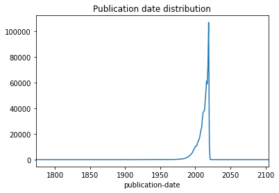
Publication Date Distribution: Most books are published in t
df["publication-date"] = df["publication-date"].astype("datetime64")
df.groupby(df["publication-date"].dt.year).id.count().plot(title='Publication date distribution')
<matplotlib.axes._subplots.AxesSubplot at 0x7f7827af68d0>
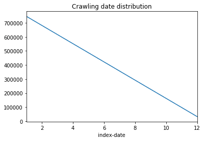
df["index-date"] = df["index-date"].astype("datetime64")
df.groupby(df["index-date"].dt.month).id.count().plot(title='Crawling date distribution')
<matplotlib.axes._subplots.AxesSubplot at 0x7f7827af61d0>
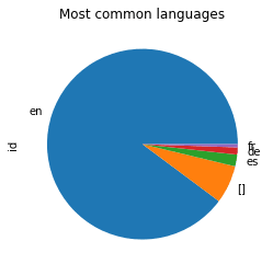
df.groupby(['lang']).id.count().sort_values(ascending=False)[:5].plot(kind='pie', title="Most common languages")
<matplotlib.axes._subplots.AxesSubplot at 0x7f78279aca58>
import math
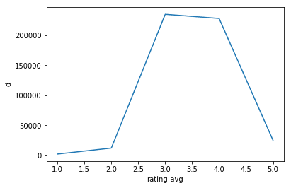
sns.lineplot(data=df.groupby(df['rating-avg'].dropna().apply(int)).id.count().reset_index(), x='rating-avg', y='id')
<matplotlib.axes._subplots.AxesSubplot at 0x7f7827970dd8>
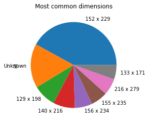
dims = pd.DataFrame({
    'dims': df['dimension-x'].fillna('0').astype(int).astype(str).str.cat(
        df['dimension-y'].fillna('0').astype(int).astype(str), sep=" x ").replace('0 x 0', 'Unknown').values,
    'id': df['id'].values
})
dims.groupby(['dims']).id.count().sort_values(ascending=False)[:8].plot(kind='pie', title="Most common dimensions")
<matplotlib.axes._subplots.AxesSubplot at 0x7f77ee8a2b38>
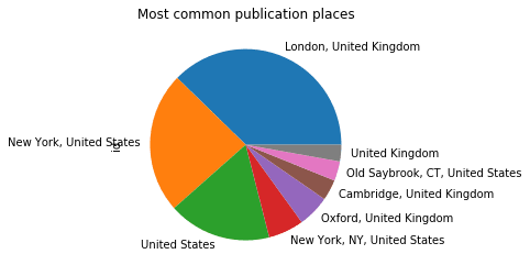
pd.merge(
    df[['id', 'publication-place']], df_p, left_on='publication-place', right_on='place_id'
).groupby(['place_name']).id.count().sort_values(ascending=False)[:8].plot(kind='pie',
                                                                           title="Most common publication places")
<matplotlib.axes._subplots.AxesSubplot at 0x7f77ee96a208>